


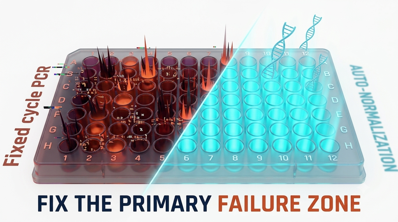
In order to sequence, you must first amplify. PCR amplification is the workhorse of library preparation. Adapter ligation is inefficient. Input is limited. Without amplification, most libraries never reach sequencing depth. You need those cycles, but they come at a cost.
Every cycle adds duplicates, chimeras, GC bias, and index-hopping artifacts. None of it is biological. All of it is baked in by the time you hand the library to the sequencer.
So, how many cycles before the data stops reflecting biology?
Nobody knows. 6, 16, 26? Whatever the protocol says? Whatever worked last time?
Too few, and your low-input wells don't make it. Too many, and your good samples are deep in the plateau, generating noise you’ll need an afternoon, a little Python, and a whole lot of heuristics to filter out. And the number that's right for well A1 is almost certainly wrong for well H12, even after you spent an hour and a half quantifying and normalizing.
That's the state of NGS library prep. Precision biology, batch amplification.
n6 started with one sole purpose: Figure out what wasn’t working in NGS and fix it. In this post, we explore the fundamental problem with library prep as we know it and what to do about it.
What are the steps involved in NGS library preparation?
Library prep turns biological material — genomic DNA, RNA, cell lysate — into something a sequencer can read. The core workflow is largely consistent across platforms, though specific steps vary by kit, application, and input type.
1. Extraction and initial QC: DNA or RNA is extracted from sample material and assessed for quantity and quality. Concentration, fragment size distribution, and integrity (RIN for RNA, DIN for DNA) all inform what comes next. This is the first moment where input variability enters the picture.
2. Fragmentation: Most sequencing platforms require fragments in a defined size range. Mechanical fragmentation (sonication, focused acoustics) and enzymatic fragmentation each produce different size distributions and end chemistries. Fragment size affects downstream amplification efficiency and library complexity, particularly in low-input workflows.
3. End repair and A-tailing: Fragmented DNA ends are polished to blunt ends, then a single adenine overhang is added to facilitate adapter ligation. Incomplete end repair is a common source of ligation inefficiency and library failure in degraded samples.
4. Adapter ligation: Platform-specific adapter sequences are ligated to fragment ends. Ligation efficiency is highly sensitive to fragment concentration, input quantity, and fragment end quality. In low-input workflows, a significant proportion of input molecules will fail to ligate successfully — meaning the material that makes it to amplification is already a fraction of what you started with.
5. Pre-amplification normalization (workflow dependent): In workflows where sample inputs are highly variable or unknown (metagenomics, mixed clinical batches, environmental samples), normalization before PCR amplification is often required to enable the use of a fixed cycle number. This typically involves bead-based normalization or quantification followed by manual dilution to a target input concentration. The goal is to level the input field so that a single cycle number produces adequate yield across all samples without overcycling the high-input ones.
6. PCR amplification: Adapter-ligated fragments are amplified to generate sufficient library material for sequencing. This is the step where library quality is most easily destroyed. Cycle number, polymerase choice, and thermal conditions all affect duplicate rate, GC representation, chimera formation, and final yield.
7. Post-amplification quantification and normalization: Amplified libraries are quantified (Qubit, qPCR, capillary electrophoresis) and normalized to a target molarity before pooling. In standard workflows, this step exists entirely to correct for the uneven amplification created in Step 6. It is time-consuming, adds reagent cost, and introduces pipetting error into the final pool.
8. Pooling and sequencing: Normalized libraries are pooled at equimolar ratios and loaded onto the sequencer. Uneven pooling — caused by imprecise normalization — results in uneven per-sample read depth, wasted sequencing capacity, and samples that fail coverage thresholds.
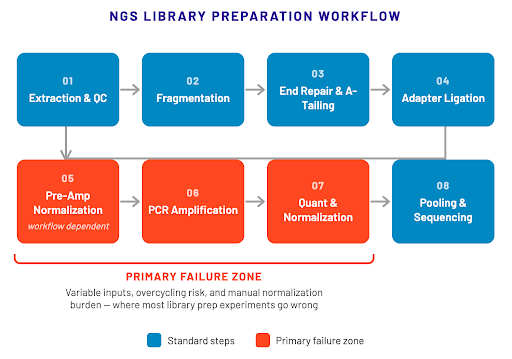
Figure 1: Workflow diagram showing all 8 steps involved in NGS library preparation. Steps 5 (pre-amplification normalization), 6 (PCR amplification), and 7 (post-amplification quantification and normalization) constitute the “Primary Failure Zone”: where variable inputs, overcycling risk, and manual normalization burden threaten the quality of your sequencing data…and your technician’s quality of life.
Explore how iconPCR™ simplifies NGS library prep workflows here.
Why is PCR amplification so problematic in library prep?
Because it's the step where a small problem becomes a big one. Fast.
PCR is exponential. That's the point. Every cycle doubles the number of molecules. Which means errors, biases, and artifacts introduced early in the amplification process are doubled right along with everything else.
Overcycling is the most common failure mode. Push a library into the plateau phase of amplification, and you get: PCR duplicates (same original molecule amplified — including any mutations introduced during amplification — into many identical copies), chimeric reads (incomplete extension products that re-anneal across templates), and GC bias (GC-rich regions amplify less efficiently, leading to coverage dropout in high-GC regions and apparent over-representation of AT-rich sequences). None of these artifacts are biologically real. All of them will be in your sequencing data.
Undercycling is the quieter failure. Insufficient amplification means inadequate library yield, which means failed samples, repeat extractions, and the worst outcome in clinical sequencing: no result.
The core problem is structural. A standard thermocycler applies a fixed cycle number to every well simultaneously. That number is chosen based on expected input and average amplification efficiency. It is optimized for the typical sample, not for each sample. On any plate with real-world input variation — which is every plate — some wells will be overcycled, and some will be undercycled. There is no cycle number that is right for all of them.
Pre-amplification normalization (Step 5 above) is the field's current answer to this problem for variable-input workflows. It reduces the spread, but it doesn’t solve the root problem — the need to adjust per sample based on what’s happening in each individual reaction — and its impact is limited because sample starting concentration does not equal target molecule concentration.
Post-amplification normalization (step 7) ensures that you have balanced libraries going into sequencing, but it doesn’t solve for the fact that each sample needed different reaction conditions in the first place.
What are the biggest challenges in NGS library preparation?
Challenge 1: The quantification and normalization tax
Consider what post-amplification normalization actually involves. Qubit fluorometry for total concentration. qPCR quantification for adapter-ligated molarity. Capillary electrophoresis for size distribution. Manual SPRI bead normalization. In many genomics core workflows, this sequence of steps takes longer than the library prep that preceded it.
And the bitter irony: you're spending that time correcting for a problem created less than an hour earlier — when your thermocycler ran the same cycle number across 96 samples that had different starting concentrations, different fragmentation profiles, and different amplification efficiencies.
The normalization tax is real: reagent cost, instrument time, technician hours, and errors that scale with every manual pipetting step. Every dilution and transfer is a chance to introduce inaccuracy into the final pool. And inaccuracy in the pool means uneven read depth in the sequencing run. (Speaking of costs, here’s what normalization is actually costing you.)
There have been attempts to speed up normalization using beads or chemistry (e.g., Normalase, Normalizer, EquiPlex), but none of them solve for the fundamental problem of over- and under-cycling.
Challenge 2: Low-input samples and sample dropout
"Low input" is a broad category. It includes single cells (picogram quantities of DNA), FFPE-derived samples (fragmented, chemically modified, often partially degraded), cell-free DNA from liquid biopsy (nanogram quantities at best, with circulating tumor DNA frequently below 1% allele frequency), and laser-capture microdissected tissue. What these samples share is this: the margin for error in amplification is extremely narrow.
A fixed cycle number calibrated for a typical input will undercycle a low-input sample. The library fails. The sample is flagged for re-extraction and re-prep — if the material even exists to re-extract. In clinical settings, a failed library isn't just an inconvenience. It's a delayed diagnosis, a repeat procedure, or a result that never comes*.
The standard workaround — run more cycles for low-input samples — directly conflicts with the equally real risk of overcycling those same samples into artifact-heavy, duplicate-saturated libraries that don't reflect the underlying biology. Low-input samples are at the intersection of both failure modes simultaneously. The conventional thermocycler has no way to navigate between them on a per-well basis.
Explore relevant data in our low-input application notes.
Challenge 3: Variable and unknown inputs — The mixed sample problem
Metagenomics and microbiome profiling present a fundamentally different version of the input variability problem: the variability doesn’t come from the lab. It is in the biology.
A 16S amplicon library prep run across 96 environmental or clinical microbiome samples will contain wells with wildly different amounts of amplifiable template, because the microbial communities themselves are different. Some species will be incredibly abundant, while others — often the most biologically significant — are rare. Each may have vastly different copy numbers of the 16s rRNA gene. None of this variability is visible prior to amplification.
When a conventional thermocycler applies a fixed cycle number to variable populations, the high-biomass samples hit the amplification plateau early and accumulate plateau-phase artifacts — chimeras, primarily — while low-biomass samples may still be in the exponential phase at cycle termination. The result: your 16S data reflects thermocycler behavior as much as it reflects microbial community composition. Chimeric sequences create taxonomic ghosts. Uneven amplification distorts relative abundance.
This is not a bioinformatics problem. It's a PCR problem. Deduplication tools and chimera-filtering pipelines can clean up the aftermath, but they can't recover information that was never captured correctly in the first place.
Dive deeper into metagenomics-specific challenges and solutions here.
Challenge 4: PCR artifacts and library fidelity
A library is supposed to represent your sample. After conventional amplification, it represents a mixture of your sample and everything PCR added to it.
Duplicates are the most visible artifact and the most discussed. PCR duplicates routinely consume 20–40% of sequencing reads in many targeted NGS workflows, with even higher duplication common in amplicon-heavy and low-complexity libraries. Post-hoc deduplication by unique molecular identifiers (UMIs) or computational deduplication helps — but it reduces effective sequencing depth. You're paying to sequence duplicates and then discarding them.
Chimeras are arguably even more damaging. A chimeric read is an artifact that looks like a real sequence — specifically, a sequence that contains elements from two different template molecules fused at a break point. In metagenomics, chimeras create false taxonomic units, inflating community diversity and generating spurious sequences that can look like novel organisms. Standard chimera-filtering pipelines catch the obvious ones; the borderline chimeras stay in the data.
GC bias affects coverage uniformity and variant detection. High-GC regions amplify inefficiently relative to AT-rich regions, leading to systematic coverage dropout at GC-rich loci — which tend to include regulatory regions, CpG islands, and certain clinically relevant gene families. Libraries with high GC bias produce less reliable variant calls in exactly the regions where accurate variant calls matter most.
Index hopping is exacerbated by over-amplified libraries. Excess free adapters in high-cycle libraries increase the probability of cross-contamination between samples sharing a sequencing lane — a problem with direct consequences for multiplexed clinical panels and multi-sample research studies.
For more on why PCR can be so problematic for library prep, watch this interview where Dr Stefan Green explains why “PCR is the enemy,” and it’s critical to amplify as little as possible to avoid PCR artifacts.
How do icon96 and icon16 instruments and iconPCR™ with AutoNorm technology address these challenges?
All of the challenges described above that make PCR a necessary evil in library preparation have two core causes:
- We know samples are variable, but we apply the same conditions to all of them.
- We don’t know what the optimal conditions are for any given sample prior to amplification.
iconPCR technology addresses both issues at once with two core innovations:
- Individual temperature control for every well for independent cycling conditions.
- Automatic adjustment of cycling conditions based on real-time amplification data.
Every well in an icon16 or icon96 instrument is monitored individually in real time. But the core innovation in iconPCR is not just that it monitors amplification in real time — qPCR machines have done that for decades. The innovation is that it acts on what it sees, at the level of each individual well.
iconPCR technology uses AutoNorm software to control cycling. AutoNorm tracks fluorescence cycle by cycle in each reaction independently. Then, when a well reaches the defined amplification threshold, that well stops cycling. Adjacent wells with lower starting input continue.
The ultimate result: High-input wells stop early. Low-input wells get the cycles they need. The plate converges on a uniform library output. Regardless of pre-amplification variability, every sample ends up at the same place because the instrument responded to each one individually.
The downstream consequences:
Pre-amplification normalization? Optional. For workflows where pre-PCR normalization was required to impose a fixed cycle number on variable inputs, iconPCR removes the underlying constraint and produces “just right” libraries regardless of initial variability. If the instrument can respond to each well individually, the premise of needing uniform input before amplification changes fundamentally.
Low-input dropout? Drastically reduced. Marginal samples that would fail under a fixed cycle number receive additional cycles without pulling high-input wells into overcycling territory. The per-well logic rescues samples at the edges of the input distribution — the ones most likely to be lost in conventional workflows.
Variable and unknown inputs? Handled by the instrument. Each well is evaluated on its own amplification curve, regardless of starting concentration. Metagenomics plates with biologically diverse inputs get per-well control rather than a plate-wide compromise. Relative abundance distortion from uneven amplification is reduced at the source, before bioinformatic correction is even needed.
Quantification and normalization tax? Eliminated. Libraries come off the instrument already normalized to a preset threshold. The post-amplification quant-and-normalize workflow collapses into a single cleanup step. No Qubit. No qPCR quant. No manual SPRI normalization. No manual pooling math.
PCR artifacts? Minimized. AutoNorm terminates each reaction in the linear phase of amplification, before plateau accumulation. Fewer plateau-phase cycles mean fewer chimeras, lower duplicate rates, less GC compression, and less excess free adapter — directly reducing index hopping risk in multiplexed runs.

Table 1: Description of key challenges that are inevitable in PCR amplification of NGS libraries by conventional workflows and comparison of how iconPCR with AutoNorm corrects for them.
See how iconPCR changes NGS library prep workflows here.
Why does adaptive amplification control matter for difficult library prep workflows?
The applications below share a common characteristic: the margin for cycling error is small, and the cost of getting it wrong is high.
FFPE-derived samples
Formalin-fixed, paraffin-embedded tissue is the most common source of archival clinical material — and one of the most challenging inputs for library prep. Formalin fixation causes DNA fragmentation and chemical modification (deamination, crosslinking) that reduce amplifiable template quantity, increase base-calling errors, and lower ligation efficiency. Starting input from an FFPE block is frequently in the low-nanogram range, with high variability between sections and cores.
Fixed cycle protocols fail FFPE samples at both ends: not enough cycles and the library is too shallow to be useful; too many cycles and a sparse, chemically damaged library is driven into the plateau where chimeras and duplicates obscure the real variants. Per-well control is particularly valuable here because it adapts to each sample's actual amplifiable template quantity rather than assuming uniform input.
See relevant data in our FFPE app note.
Liquid biopsy — cfDNA and ctDNA
Cell-free DNA (cfDNA) is present in plasma at very low concentration, typically only a few nanograms per milliliter in healthy individuals. The tumor-derived fraction (ctDNA) may comprise less than 0.1% of total cfDNA, particularly in early-stage disease or minimal residual disease, making highly sensitive workflows essential for reliable detection.
Library prep for liquid biopsy operates at the absolute limit of input sensitivity. Adapter ligation efficiency, amplification fidelity, and duplicate rate are all critical determinants of whether a low-frequency variant is detected or missed.
Overcycling a cfDNA library inflates duplicate rates in an already sparse library, reducing effective unique molecule coverage. Undercycling produces insufficient yield for sequencing. The difference between these two failure modes may be two or three cycles — a margin that a fixed-cycle conventional thermocycler cannot reliably hit across a plate of variable-concentration plasma samples.
Watch a webinar on cfDNA sequencing at Dana-Farber Cancer Institute.
Single-cell RNA sequencing
Single-cell workflows are defined by extreme input variation. Individual cells vary enormously in RNA content, capture efficiency, and cDNA synthesis yield. A plate designed for single-cell library prep will routinely contain wells representing high-quality cells with thousands of detected genes alongside wells containing empty droplets, dead cells, or low-RNA-content cell types.
A conventional thermocycler applies one cycle number to all of them. High-quality cell wells are pushed into overcycling. Marginal wells are undercycled and dropped. Per-well control collapses this variance: each well gets the amplification it needs, productive wells aren't over-amplified, and the per-cell library quality becomes a function of biology — not the plate position.
Metagenomics and 16S amplicon sequencing
As described above, community biomass variation is intrinsic to metagenomics experiments. 16S amplicon workflows are particularly sensitive to chimera formation, which occurs predominantly in the plateau phase. Per-well control reduces chimera generation by stopping each reaction before plateau accumulation, directly improving the accuracy of community composition estimates.
For shotgun metagenomics, even low levels of overcycling in high-biomass wells produce enough PCR artifacts to distort taxonomic assignments and relative abundance calculations. When accurate ecology is the endpoint, the quality of the amplification step has direct scientific consequences.
Learn how to combine long-read sequencing with iconPCR for greater metagenomic insights in this webinar.
Low-input clinical sequencing panels
Targeted clinical sequencing (oncology panels, pharmacogenomics, hereditary risk panels) runs on input material that is frequently heterogeneous in quality and quantity. Clinical labs processing high volumes of FFPE, biopsy, and needle aspirate material see consistent variability in library yield that requires manual flagging and intervention in conventional workflows. Per-well normalization reduces that intervention burden, improves first-pass success rates, and increases sample throughput without sacrificing data quality.
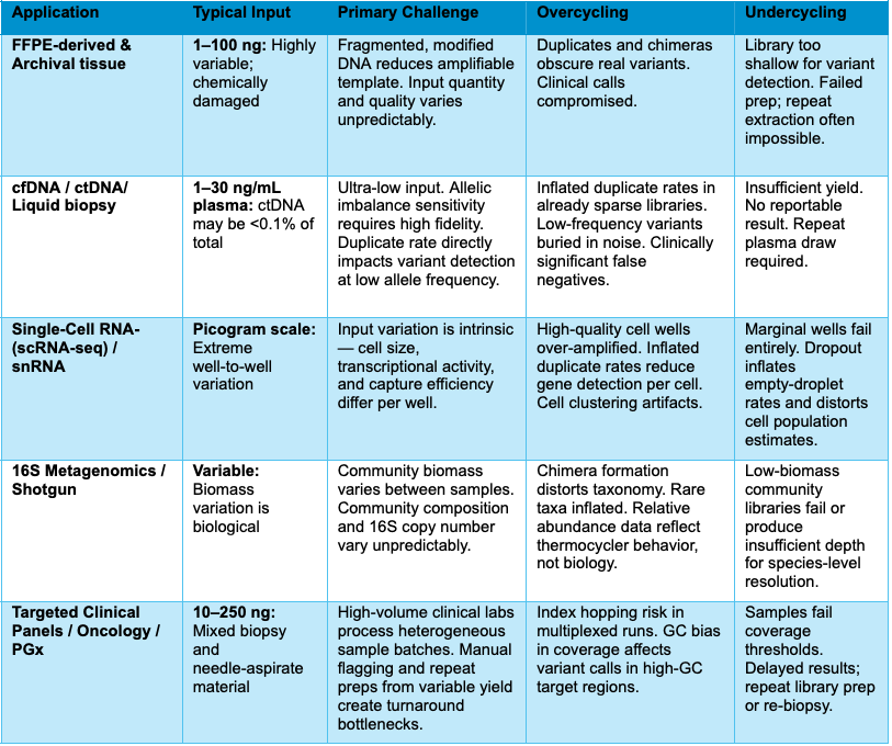
Table 2: Summary of how over- and under-cycling negatively impacts library preparation for particularly challenging sequencing applications.
Your library is telling the sequencer a story. Make sure it's the right one. Talk to an n6 application scientist.
FAQ
What steps are involved in NGS library preparation?
NGS library preparation typically includes: (1) sample extraction and QC, (2) fragmentation, (3) end repair and A-tailing, (4) adapter ligation, (5) pre-amplification normalization (in variable-input workflows), (6) PCR amplification, (7) post-amplification quantification and normalization, and (8) pooling and sequencing.
How many PCR cycles should I use for NGS library prep?
The optimal PCR cycle number depends on input quantity, adapter ligation efficiency, and the specific library prep kit. Most workflows recommend the minimum number of cycles required to achieve target yield — typically 6–15 cycles for standard gDNA inputs, more for low-input or degraded samples. Using too many cycles drives libraries into the plateau phase, generating duplicates, chimeras, and GC bias. The challenge is that the optimal cycle number varies across wells on the same plate — a problem that per-well-controlled instruments like iconPCR address directly.
What causes PCR duplicates in NGS libraries?
PCR duplicates arise when the same original library fragment is amplified into multiple identical copies. They accumulate preferentially in the plateau phase of amplification — when all templates have been copied and continued cycling produces diminishing returns. High duplicate rates reduce effective sequencing depth and inflate cost. The primary driver is overcycling: running more cycles than the reaction needs. Per-well cycle control reduces duplicates by stopping each reaction at the late exponential phase rather than driving it into the plateau.
How do I normalize libraries for sequencing?
Standard library normalization involves quantifying each amplified library (by Qubit, qPCR, or capillary electrophoresis), calculating molar concentration based on fragment size, and diluting each library to a common target molarity before pooling. This process is time-consuming and introduces pipetting error into the final pool. iconPCR with AutoNorm normalizes libraries during amplification — stopping each well at a defined threshold — so post-amplification normalization is eliminated or greatly simplified.
What is the best library prep approach for low-input samples?
Low-input library prep requires maximizing ligation efficiency, minimizing sample loss at each step, and carefully controlling PCR cycle number to balance yield against artifact generation. For samples like FFPE, cfDNA, or single cells, the window between undercycling (failed library) and overcycling (artifact-heavy library) is narrow. Per-well amplification control — as in iconPCR — allows low-input wells to receive additional cycles without driving high-input wells into overcycling, improving first-pass success rates across heterogeneous sample sets.
How does overcycling affect sequencing data quality?
Overcycling pushes PCR amplification into the plateau phase, where incomplete extension products accumulate and re-anneal across templates to form chimeric molecules. It also drives exponential duplication of existing library fragments, increases GC bias through differential template re-amplification, and generates excess free adapter sequences that contribute to index hopping in multiplexed runs. These artifacts can inflate diversity estimates, distort relative abundance calculations, reduce effective sequencing depth, and introduce false-positive variant calls — all without being immediately obvious in the raw data.
What is AutoNorm and how does it work in library prep?
AutoNorm is n6's per-well amplification control technology built into the iconPCR instrument. Each well has an individual optical sensor that monitors fluorescence in real time, cycle by cycle. When a well reaches the defined amplification threshold — indicating the reaction has reached the late exponential phase — that well stops cycling automatically, while adjacent wells continue if they need more cycles. The result is a plate of libraries that all converge on the same amplification endpoint, eliminating the need for post-amplification quantification and manual normalization.
Can iconPCR instruments handle FFPE or cfDNA samples?
Yes. FFPE and cfDNA samples are among the applications that benefit most from per-well amplification control, precisely because input quantity and amplification efficiency are highly variable in these sample types. iconPCR's ability to give low-input wells additional cycles — without overcycling high-input wells on the same plate — directly addresses the failure modes most common in FFPE and liquid biopsy library prep workflows.
How do I reduce PCR artifacts in metagenomics library prep?
The primary strategy for reducing chimera formation and abundance bias in metagenomics library prep is to minimize PCR cycle number — running the fewest cycles that produce adequate yield. In practice, this is difficult to implement on a conventional thermocycler across a plate of samples with variable community biomass. iconPCR stops each well at the late exponential phase regardless of starting biomass, reducing plateau-phase chimera generation and uneven amplification across the plate. This improves both the accuracy of community composition estimates and the efficiency of post-sequencing chimera filtering.
*For Research Use Only. Not for use in diagnostic procedures. iconPCR™ products are intended for laboratory research applications only and have not been validated for clinical diagnostic use.


