The below post is an in-depth overview of challenges and solutions involved in NGS library preparation for microbial samples that will be informative for researchers who are relatively new to 16s rRNA or shotgun metagenomic sequencing. For experts in the microbiome sequencing space, we recommend navigating directly to one of the following data-rich resources:

• Metagenomics sequencing application note
• Poster: 16S Workflow and Data Quality Improvements Using iconPCR Demonstrates Higher Biological Resolution from Metagenomic Soil Samples
• Publication: Cryptic Insect Microbiome Compositions Unveiled with Full-Length 16S Sequencing
• Publication: Applying PCR cycle autonormalization to improve PacBio full-length 16S rRNA sequencing
• Publication: Using carrier DNA in ultra-low input library preparations for metagenomic sequencing

Publication: The use of iconPCR for 16S library preparation improves data quality and workflow

Typical NGS workflows don’t cut it for metagenomics

Microbiome sequencing has a reputation problem.

From the outside, it looks like one of the most powerful tools in modern biology: sequence everything in a sample and reconstruct the microbial world inside. No culturing. No assumptions. Just data.

But anyone who’s actually run these workflows knows the reality is messier. A lot messier.

Microbial samples are fundamentally different from the tidy, single-organism inputs many NGS workflows were built around. Instead of a uniform population, you’re dealing with highly heterogeneous communities, where composition, concentration, and complexity can vary dramatically—not just between studies, but from sample to sample within the same experiment.

In one tube, you might have a relatively balanced microbial community. In the next, a single organism dominates 90% of the sample. In another, total DNA concentration (let alone 16s rRNA concentration specifically) is barely detectable, but the biological diversity is high. And in many cases, you don’t know which scenario you’re dealing with until it’s already too late.

That uncertainty creates cascading problems downstream.

It’s impossible to predict the perfect number of cycles for library amplification when template abundance spans orders of magnitude. Highly abundant taxa amplify aggressively, while rare organisms struggle to be detected at all. Library yields become inconsistent. Some samples sail through prep with high concentrations, while others barely produce enough material to sequence. And because most workflows rely on post-PCR quantification and normalization, all of that variability gets pushed into a manual, time-consuming bottleneck.

By the time your libraries hit the sequencer, the biological signal has already been reshaped by the workflow itself.

Video Caption: Kerry Hair from Penn State Genomics Core Facility discusses critical data that is often missed in conventional microbiome sequencing. Read the blog: “Discoveries at the Margins: How iconPCR™ is Transforming Amplicon and Microbiome Workflows at Penn State”.

16S rRNA sequencing vs. shotgun metagenomics: Choosing the right tool

Before optimizing a workflow, it’s worth stepping back and asking a more fundamental question: what kind of sequencing do you actually need?

Both 16S rRNA sequencing and shotgun metagenomics aim to characterize microbial communities, but they do so in fundamentally different ways. Those differences have real implications for workflow complexity, cost, and data interpretation.

16S rRNA sequencing targets a conserved genetic marker present in bacteria and archaea. By amplifying and sequencing this region, you can infer the taxonomic composition of a sample without sequencing entire genomes. It’s efficient, scalable, and well-suited for studies where the primary goal is to understand who is there.

Shotgun metagenomics, on the other hand, sequences all DNA in the sample. That includes microbial genomes, host DNA, and everything in between. The payoff is higher resolution—you can often get down to species or even strain level, and you can start to infer functional potential. But that added depth comes at a cost: more complex workflows, higher sequencing requirements, and increased sensitivity to upstream variability.

In practice, 16S remains the workhorse for many applications, especially when throughput and cost matter. Shotgun approaches become valuable when resolution is critical or when functional insights are required. As the more popular workflow, we’ll speak primarily to 16S      here, but the workflow improvements we’ll explore apply to shotgun metagenomics as well.

16S vs. Shotgun Metagenomics

16S and shotgunsequencing are both highly sensitive to initial sample variability

The 16S library prep workflow—And where it quietly fails

On paper, the 16S workflow is straightforward: extract DNA, normalize samples for total DNA, amplify the 16S region, prepare libraries, normalize again, and sequence. Each step is well understood. Each has established protocols.

And so, we take for granted that the outcome represents actual biology. The problem is, each step amplifies variability introduced in the previous one.

PCR is the most critical inflection point. Because amplification efficiency depends on template abundance, even small differences in starting composition can lead to large differences in output. Rare taxa risk dropping out entirely, while dominant organisms become even more dominant. At the same time, PCR artifacts accumulate as cycle number increases. These artifacts, which include mutations, primer dimers, and chimeric molecules, can be difficult to identify until after sequencing.

Library preparation introduces another layer of variability. Adapter ligation or indexing efficiency can differ across samples, further widening the gap in library concentrations.

But the biggest pain point is normalization. Most workflows treat it as a downstream fix: measure each library, calculate concentrations, and manually adjust volumes to equalize input for sequencing. It’s slow, labor-intensive, and inherently error-prone.

More importantly, it’s reactive. By the time you’re normalizing, the underlying variability has already shaped your libraries. And normalizing for total DNA before amplification just adds labor without actually solving the problem, because total DNA does not equal target DNA; the number of copies of the 16S rRNA genes can vary dramatically from species to species.

How to speed up your 16S rRNA sequencing workflow (without cutting corners)

When people talk about speeding up sequencing workflows, they often focus on automating pipetting. That’s because there are a lot of small, manual steps.

Let’s review them again: quantifying DNA, adjusting volumes, amplifying, measuring again, recalculating concentrations, normalizing—not to mention re-running failed samples. Individually, each step feels manageable. Together, they add hours or days to a workflow.

But the most effective way to speed things up isn’t to optimize steps. It’s to remove them entirely.

This is where PCR-based normalization strategies start to change the game. Instead of amplifying samples and then correcting for variability afterward, these approaches aim to control output during amplification itself. By tuning PCR conditions—particularly cycle number—samples can be driven toward a more uniform endpoint.

That means fewer downstream adjustments, fewer opportunities for error, and a significantly shorter path from sample to sequencing.

See how PCR-based normalization is transforming metagenomics from soil to spacecrafts in this blog.

Technologies for normalization in 16S library prep: What actually moves the needle

There’s no shortage of ways to prepare a 16S library. Most workflows look different on the surface—different kits, different cleanup steps, different instruments—but under the hood, they tend to fall into a few familiar categories.

Bead-based normalization methods aim to standardize DNA concentrations through binding capacity. Enzymatic approaches attempt to equalize libraries chemically. These can streamline parts of the workflow, but they still operate as add-ons—additional steps layered onto an already complex process.

What’s more powerful is a shift toward integration, where normalization is no longer a separate task but a built-in feature of amplification itself.

That’s where AutoNorm™ technology comes in. AutoNorm embeds normalization into the amplification step. Using real-time signals, AutoNorm stops cycling and enters a cold hold when target amplicon concentration is reached. Importantly, AutoNorm functions within iconPCR™  thermocyclers that have individually controlled wells (16 or 96), such that cycle number can vary down to the individual well level. The result is samples that are normalized during PCR without being under or over amplified.

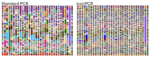
It’s not just a faster process (eliminating normalization steps before and after library amplification) but a more consistent one. Libraries enter sequencing with tighter concentration distributions and reduced variability and PCR artifacts across samples.

In a proof-of-concept study, full-length and variable region 16S      libraries that were Auto     Normalized by iconPCR exhibited cleaner Bioanalyzer profiles, a statistically significant reduction in chimeras, and richer species diversity. Read the pre-print here.

16S Library prep normalization approaches compared

Why normalization is so important for metagenomic sequencing

Normalization is often treated as a technical step—something you do because the protocol says so. But in metagenomics, it plays a much bigger role. It’s the gatekeeper between your library prep and your sequencing data, and it directly determines how sequencing capacity is allocated across samples.

When normalization is off, everything downstream suffers.

Samples with higher concentrations consume a disproportionate share of sequencing reads. Lower-concentration samples get under-sequenced, sometimes to the point where meaningful analysis becomes impossible. The result is uneven coverage, distorted relative abundances, and unreliable diversity metrics.

What makes normalization particularly challenging in metagenomics is that it’s trying to correct for upstream variability that spans multiple dimensions: variability in microbial communities, total DNA input, 13 rRNA gene copy number, amplification efficiency, and library prep yield. Traditional methods—whether based on fluorescence quantification or qPCR—can measure concentration (to a point), but they don’t address the root cause of variability. They simply redistribute it.

This is why normalization becomes such a bottleneck. It’s not just time-consuming; it’s fundamentally limited in how much it can fix.

In contrast, AutoNorm controls variability during PCR to address variability at its source, instead of measuring and correcting for it after the fact. When libraries exit amplification with similar effective concentrations, normalization becomes trivial or unnecessary.

In practice, this shift has measurable effects. Studies incorporating iconPCR with AutoNorm have shown:

• More uniform read distribution across samples
• Reduced need for re-sequencing underrepresented libraries
• Improved reproducibility between runs

Stefan Green discusses how the Rush University Core Facility avoids normalizing 1,000s of samples for 16S amplicon sequencing all while reducing PCR artifacts such as chimeras. Learn more in this blog.

Improving Shannon Diversity Index (without distorting the biology)

The Shannon Diversity Index is one of the most widely reported metrics in microbiome studies—and one of the most misunderstood.

At its core, it captures two things: how many taxa are present, and how evenly they’re represented. In theory, it’s a property of the biological sample. In practice, it’s heavily influenced by the workflow used to generate the data.

This is where things get tricky.

A low Shannon Index doesn’t necessarily mean low biological diversity. It can just as easily reflect technical bias. If PCR preferentially amplifies dominant taxa, or if normalization fails to equalize sequencing depth across samples, the resulting data will appear less diverse—even if the underlying community is rich and complex.

In workflows that improve amplification uniformity and reduce variability in library preparation, the effects show up clearly in diversity metrics. More even representation of taxa leads to higher observed diversity, particularly through better detection of low-abundance organisms.

In evaluations of integrated 16S library prep workflows, these improvements aren’t just theoretical. Samples processed AutoNorm consistently show:

• Increased evenness in taxonomic distribution
• Greater detection of rare taxa
• Higher overall diversity indices

The important distinction is that these gains reflect better measurement of the same biology, not artificial inflation.

Increasing taxonomic diversity and managing low input in shotgun sequencing

While 16S workflows have their own challenges, shotgun metagenomics amplifies them.

Because shotgun sequencing captures all DNA in a sample, it’s particularly sensitive to imbalances—both biological and technical. Host DNA contamination can dominate reads. Highly abundant microbial genomes can overshadow rare species. Library prep bias can skew representation before sequencing even begins.

The instinctive solution is often to sequence deeper. And while increased depth can help, it’s not a complete fix. If your library is biased going in, you’re just collecting more biased data.

Improving taxonomic diversity in shotgun workflows requires attention to both sample preparation and library construction.

Host depletion strategies can reduce background noise, freeing up sequencing capacity for microbial DNA. Fragmentation methods can influence how evenly genomes are represented. But without careful control of amplification, bias is inevitable. Ensuring that libraries are balanced by avoiding under and over cycling before sequencing helps prevent dominant samples from consuming disproportionate reads, allowing more equitable detection of taxa across the dataset.

Another frequent challenge in shotgun metagenome sequencing of environmental samples is ultra-low input DNA—     frequently 10 pg or less, making fluorometric quantification difficult. Without quantification, it’s impossible to know how many cycles to use for library amplification.

In a recent study by the Rush University Core Facility, a method was developed for sequencing libraries from down to 50 fg      of input DNA using spike-in exogenous carrier DNA. Critically, the team employed AutoNormalization with iconPCR to dynamically cycle until a library concentration sufficient for sequencing was reached.

Under normal library prep conditions, duplication rates from the spike-in DNA would have masked any real signal from the target sample, but with AutoNorm, data loss due to PCR duplication is reduced thanks to adaptive cycling. Get the full method in the pre-print here.

Methods to increase taxonomic diversity in shotgun sequencing

Case Study: AutoNormalization in PacBio full-length 16S sequencing improves yield and data quality

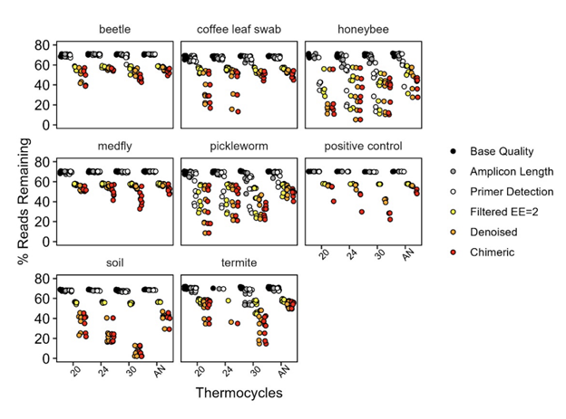
In a recent study analyzing microbial communities in agriculturally important environmental samples, researchers at the USDA specifically tested Auto-Normalization by iconPCR versus fixed cycle protocols.

Autonormalization came out on top by almost every measure. It produced the most usable reads after quality control (11.3M vs 8.9M, 7.3M, and 8.1M for 30-, 24-, and 20-cycle fixed protocols, respectively). More importantly, it produced the most even distribution of reads across samples — a key advantage when pooling diverse specimen types.

The 30-cycle protocol, by contrast, was a consistent underperformer despite generating a similar raw read count, losing disproportionate numbers of sequences during denoising and chimera removal.

The penalty for overamplification was most severe in high-diversity samples. Soil samples, the most diverse, retained fewer than 10% of reads through the full pipeline at 30 cycles. Substitution errors also scaled with cycle number, though even at 30 cycles the absolute rates remained low.

Critically, none of the protocols meaningfully distorted community composition: specimen type dominated the beta-diversity signal regardless of how samples were amplified, which is reassuring for anyone worried that switching protocols might change their biological conclusions.

Access the full preprint here.

FAQ: Metagenomics & 16S Sequencing

What is 16S rRNA sequencing used for?
It’s used to profile bacterial and archaeal communities by targeting a conserved gene that enables taxonomic identification.

How do I speed up my 16S rRNA sequencing workflow?
The most effective way is to eliminate bottlenecks like quantification and normalization by integrating them into earlier steps such as PCR. Learn how you can speed up your library preparation workflow here.

How do I reduce the cost of metagenomic sequencing?

Removing manual normalization and quantification steps can reduce library preparation costs by 50% or      more. Calculate how much you could save in your sequencing workflow here.

What technologies are available for 16S library prep?
Options include traditional workflows, bead-based normalization, enzymatic methods, and integrated PCR-based approaches that combine amplification and normalization.

What is the best way to normalize samples for metagenomic sequencing?
Approaches that reduce manual handling and control variability earlier in the workflow—particularly during amplification—tend to produce the most consistent results.

How does normalization affect sequencing results?
It determines how sequencing reads are distributed across samples, directly impacting data quality, coverage, and diversity metrics.

How do you improve Shannon Diversity Index?
By reducing technical bias—especially in PCR and library prep—and ensuring even representation of taxa across samples.

What reduces taxonomic diversity in sequencing?
Uneven amplification, poor normalization, sequencing depth imbalance, and sample contamination can all reduce observed diversity.

Is shotgun sequencing better than 16S?
Not inherently. Shotgun offers higher resolution, but 16S is often more efficient and scalable depending on the research goal.

What is PCR bias in microbiome sequencing?
It refers to preferential amplification of certain DNA sequences, which can distort the apparent composition of a microbial community.

What is full-length 16S sequencing?
It involves sequencing the entire 16S gene, providing higher taxonomic resolution compared to short-read approaches.

How many reads do I need for metagenomics?
It depends on sample complexity, but insufficient depth can limit detection of low-abundance organisms.