


This guide is a full overview of cfDNA and liquid biopsy sequencing workflows, written for researchers and core facility teams building or improving a targeted cfDNA assay. If you already run cfDNA panels and want data first, go straight to these resources:
Application note: Sensitive cfDNA Sequencing at Scale with icon96
Webinar: How to optimize low-input cfDNA library prep for targeted sequencing sensitivity
Amplified Voices: Zach Herbert, Dana-Farber Cancer Institute
Poster: Reducing amplification bias in NGS-based MRD assays using adaptive PCR cycle normalization
What is cfDNA sequencing, and why is it different from every other NGS workflow?
Cell-free DNA (cfDNA) sequencing is the targeted or genome-wide analysis of short DNA fragments circulating in plasma, most commonly to detect tumor-derived variants for minimal residual disease monitoring, treatment response tracking, or early detection. The circulating tumor DNA (ctDNA) subset of that pool is what carries the signal.
What makes cfDNA different is not the chemistry. It’s the math.
Most NGS workflows have more input material than they need. cfDNA workflows almost never do. Healthy plasma typically carries roughly 1 to 10 ng of cfDNA per mL (Frontiers/PMC review of cfDNA origins), and a broad survey of healthy donors put the average near 6 ng per mL of plasma (PLOS ONE, Parpart-Li et al.). Those fragments are short and uniform, with a modal length near 167 bp reflecting their nucleosomal origin (Snyder et al., Cell).
And the fraction you actually care about is smaller still. ctDNA commonly represents under 1% of total cfDNA in early-stage disease, and can sit well below 0.1% (Cancer Biology & Medicine review).
So the honest framing for a cfDNA assay is this: you are not sequencing a sample, you are counting molecules. Every step that loses, duplicates, or distorts a molecule directly costs you sensitivity. That includes PCR.
Why input mass, not sequencing depth, sets your detection floor
Short answer: sequencing deeper cannot recover a variant molecule that was never in the tube. Input mass determines the number of unique template molecules available, and that number sets the theoretical limit of detection before a single read is generated.
A haploid human genome is roughly 3.3 pg of DNA. That converts input mass into something far more useful than nanograms: genome equivalents (GE).
Read the upper-left corner of that table carefully. At 1 ng input, which the Dana-Farber team describes as roughly 300 genome equivalents, a 0.1% variant is expected to appear as a fraction of a molecule (SelectScience webinar summary). No amount of sequencing depth fixes that. No informatics pipeline fixes that.
This is why cfDNA assay design is fundamentally a molecule-preservation problem, and why the Dana-Farber Molecular Biology Core Facilities (MBCF) publishes explicit input-to-sensitivity guidance rather than a single headline LoD: their internal validation supports reliable detection near 0.5% VAF at 1 ng and near 0.25% VAF at 10 ng, with ultra-sensitive targets below 0.1% requiring substantially more input (MBCF cfDNA service page).
The practical implication: if your assay is losing molecules during library prep, you are not running the assay you validated. You are running a lower-sensitivity version of it.
Where cfDNA library prep actually fails
Short answer: the four highest-risk steps are extraction recovery, adapter ligation efficiency, PCR amplification, and hybrid capture. Of those, PCR is the only one that can both destroy information and hide the evidence until after sequencing.
Here is the standard targeted cfDNA workflow and the failure mode that lives inside each step.
1. Plasma processing and extraction. Delayed processing allows leukocyte lysis, which floods the sample with genomic DNA and dilutes the ctDNA fraction. Longer fragments in your trace are a warning sign, not a bonus.
2. Adapter ligation with dual UMIs. This is the conversion step. Every original molecule that fails to ligate is permanently gone. Ligation efficiency also varies sample to sample, which means two tubes with identical input masses can enter PCR with significantly different molecule counts.
3. PCR amplification. This is the inflection point, and we will spend most of this guide here.
4. Hybrid capture and pooling. Capture efficiency and pool balance decide how much of your sequencing budget lands on target versus off target. Imbalanced pools mean some samples are over-sequenced while the samples that need depth get starved.
5. Sequencing and duplex consensus calling. Powerful error suppression, but strictly downstream. It filters noise. It cannot manufacture signal.
We have written more broadly about how these failures compound in Better libraries, better biology: solving the hidden failures of NGS library prep.
Why fixed-cycle PCR is the wrong tool for cfDNA
Short answer: fixed-cycle PCR applies one cycle number to every well, which means it is simultaneously wrong for the low-input samples and wrong for the high-input samples on the same plate.
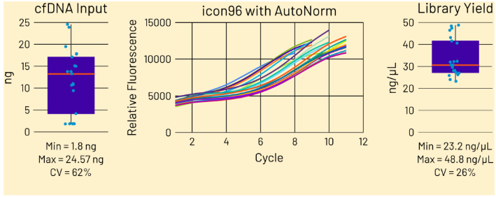
A conventional thermocycler runs a number that a user picked from a protocol. It has no feedback, no per-well awareness, and no way to respond to what is actually happening in each reaction. Apply that to a plate of patient plasma samples spanning 2 to 25 ng, and two things happen at once.
Under-amplified wells produce insufficient library mass for hybrid capture. They drop out of the pool, get flagged for repeat, and consume irreplaceable sample.
Over-amplified wells are the more dangerous failure, because they look fine. Once a reaction runs past the linear phase into plateau, you are no longer amplifying information. You are amplifying copies of copies. PCR duplicate rate climbs, effective coverage falls, polymerase errors and chimeric molecules accumulate, and the duplex families you depend on become distorted rather than informative.
The literature is direct about this. Reducing DNA input reduces library complexity and measurably degrades variant detection, because PCR cannot create more information than was present in the original template (Journal of Molecular Diagnostics, via PubMed). And PCR duplicate rate is driven primarily by the ratio between library complexity and sequencing depth (Molecular Ecology Resources). In a molecule-limited workflow, that ratio is exactly what you cannot afford to get wrong.
The result is a workflow where library yield varies wildly across a plate for reasons that have nothing to do with biology. In the Dana-Farber work, standard fixed-cycle amplification produced a 54% coefficient of variation in library yield across identical 10 ng inputs (n6 low-input and degraded samples page).
That is a 54% CV from samples that were, by design, the same. Every bit of that variance is workflow noise sitting on top of the biological signal you are trying to measure.
We go deeper on this failure mode in You can't normalize your way out of a bad PCR in NGS library prep.
UMIs and duplex sequencing are essential, and they are not enough
Short answer: duplex sequencing suppresses errors with extraordinary power, but it operates on the molecules that survived library prep. It improves specificity. It cannot restore sensitivity that PCR already cost you.
Duplex sequencing tags both strands of an original DNA duplex and calls a variant only when it appears on both strands. The original method described a theoretical background error rate below one artifactual mutation per billion nucleotides sequenced (Schmitt et al., PNAS). In practice, the Dana-Farber workflow describes duplex consensus calling, reducing the effective error rate from roughly 10⁻³ to 10⁻⁴ down to roughly 10⁻⁶ to 10⁻⁷, a 100- to 1,000-fold improvement (MBCF cfDNA service page).
That is a remarkable specificity gain. It is also, structurally, a filter.
To call a duplex consensus, you need reads from both strands of the same original molecule. If over-amplification skews family sizes so that some molecules dominate the read pool while others are represented once or not at all, you lose duplex families. If under-amplification starves the library, you never had enough molecules to build families from in the first place.
The framing that matters: UMIs and duplex calling protect you from errors. Amplification control protects you from losses. You need both, and only one of them is usually being managed.
The on-target rate problem nobody budgets for
Short answer: in targeted cfDNA panels, on-target percentage is a direct multiplier on your effective sequencing spend, and it degrades when input pools are unbalanced.
If your on-target rate is 70%, three out of every ten reads you worked for landed somewhere you do not care about. Push that to 90%, and you have effectively increased your usable depth by nearly 30% without buying a single additional read.
Pool balance is a large part of what drives this. When library concentrations across a pool vary by several-fold, the pooling math becomes an estimate, and the samples that most needed coverage are frequently the ones that get the least. In the Dana-Farber workflow, moving to sample-specific amplification took on-target rates from approximately 70% to above 90% across both 1 ng and 10 ng inputs (SelectScience webinar summary).
For context on what unbalanced pools and failed runs actually cost a lab, see The real cost of NGS failure.
What changes when amplification itself is controlled
Short answer: real-time, per-well PCR control stops every reaction at its own optimal endpoint, which normalizes library yield during amplification instead of correcting for it afterward.
iconPCR with AutoNorm monitors fluorescence in each of 96 independently controlled wells, cycle by cycle, and terminates each reaction when it reaches a defined threshold. Low-input wells get the cycles they need. High-input wells stop before they run into plateau. Every well is treated as its own experiment, because it is.
Three things follow from that, and they matter specifically for cfDNA.
Mixed-input runs become possible. You no longer need to batch samples by input amount across separate thermocycler runs. Dana-Farber co-processed 1 ng and 10 ng samples in a single run, and processed roughly 100 patient-derived cfDNA samples spanning 2 to 25 ng together (SelectScience webinar summary).
Pre-pooling quantification comes out of the workflow. If libraries exit PCR at comparable concentrations, the quantify-calculate-dilute-pool loop stops being a bottleneck. For labs running precious plasma samples, this also means fewer handling steps and less material consumed on QC.
Over-amplification stops being invisible. Every well produces an amplification curve. The black box becomes a record. As Zach Herbert put it in the webinar: "icon96 is really a game changer, shining a light into that black box [of PCR]. We can now see exactly the amplification path of every sample."
For a full comparison against enzymatic and bead-based normalization approaches, see The Great NGS Library Normalization Showdown.
Case in point: the Dana-Farber cfDNA workflow
Short answer: the Molecular Biology Core Facilities at Dana-Farber Cancer Institute built a targeted cfDNA service around dual-UMI ligation, real-time PCR normalization on icon96, co-optimized hybrid capture, and duplex consensus calling.
The MBCF workflow runs in four stages (MBCF cfDNA service page):
- Adapter ligation using the IDT xGen cfDNA and FFPE DNA Library Preparation Kit, selected for ligation efficiency with low-input and fragmented DNA, with dual UMIs labeling both strands of each original molecule.
- PCR amplification on icon96, where fluorescence is monitored in real time, and amplification terminates automatically when each sample reaches a defined threshold, compensating for variable input and variable ligation efficiency.
- Hybrid capture against custom biotinylated panels, with probe design, hybridization, and wash stringency co-optimized to achieve on-target rates above 90%.
- Sequencing on NovaSeq X Plus with duplex consensus calling, where a variant is called only when present on both strands of an original molecule.
Reported results
Sources: n6 low-input and degraded samples page, SelectScience webinar, MBCF cfDNA service page. These results describe the Dana-Farber MBCF workflow specifically, under the panel, chemistry, and sequencing conditions used there.
Hear the full workflow in Zach Herbert's own words on Amplified Voices or in the on-demand webinar.
Why this matters more as MRD monitoring scales
Short answer: MRD is the application where sensitivity, reproducibility, and throughput all become non-negotiable at once, and it is growing fast.
ctDNA-based molecular residual disease testing is now an established prognostic tool in colorectal cancer, with large prospective analyses such as GALAXY demonstrating its association with recurrence risk (Nature Medicine). Serial monitoring means the same patient is sampled repeatedly over time, which means run-to-run variability is no longer a nuisance. It is a confounder that can look like biology.
If your library prep introduces a 54% yield CV, longitudinal comparisons inherit that noise. If your assay silently over-amplifies a subset of timepoints, apparent changes in variant fraction may reflect amplification behavior rather than tumor dynamics. Reproducibility is the whole product in serial monitoring, and reproducibility is decided during amplification.
The broader liquid biopsy market is projected to reach roughly $7.05 billion by 2030 at an 11.8% CAGR (MarketsandMarkets). The labs that scale successfully will be the ones whose per-sample workflow does not require per-sample babysitting.
See our poster on reducing amplification bias in NGS-based MRD assays using adaptive PCR cycle normalization.
A practical checklist for designing a cfDNA sequencing workflow
Use this as a design review for a new assay or an audit of an existing one.
Define sensitivity in molecules, not percentages. Before selecting a panel, state the target VAF and back-calculate the input mass required to expect a countable number of mutant molecules. If the math does not work, no downstream choice will rescue it.
Protect conversion efficiency. Choose a ligation chemistry validated for low-input, fragmented DNA. Measure conversion, not just yield.
Stop treating cycle number as a protocol constant. It is the single most consequential variable in a molecule-limited workflow, and it should be determined by the reaction, not by the protocol author.
Eliminate pre-pooling quantification where you can. Every QC step on a precious sample is material spent on measurement rather than on data.
Balance pools during amplification, not after it. Post-PCR normalization equalizes concentration. It does not equalize information.
Visualize your amplification. If you cannot see the amplification curve for every well, you cannot distinguish a low-signal sample from a failed reaction.
Validate sensitivity across your real input range. Reference standards at a single input do not predict performance on patient plasma spanning an order of magnitude.
Frequently asked questions
What is the difference between cfDNA and ctDNA?
cfDNA is all cell-free DNA circulating in plasma, most of it from normal hematopoietic cells. ctDNA is the tumor-derived subset of that pool. In early-stage disease, ctDNA often represents under 1% of total cfDNA, and can fall below 0.1% (Cancer Biology & Medicine).
How much cfDNA can I expect from a plasma sample?
Healthy individuals typically yield roughly 1 to 10 ng of cfDNA per mL of plasma, with reported averages near 6 ng per mL (PLOS ONE). Cancer patients generally have higher concentrations, but the range is wide and sample-dependent.
Why are cfDNA fragments about 167 bp long on average?
Plasma cfDNA is cut by nucleases at the exposed DNA between nucleosomes, so fragment length is set by how much DNA is physically shielded from digestion. The nucleosome core protects about 147 bp. A linker histone binds roughly 20 bp more at the DNA entry and exit points, forming a chromatosome, and 147 plus that linker segment is what produces the ~167 bp peak. Snyder et al. found the dominant peak in plasma cfDNA sits at ~167 bp, matching the chromatosome rather than the bare nucleosome, with a secondary ~147 bp population from nucleosomes without the linker histone (Snyder et al., Cell).
How many PCR cycles should I use for cfDNA library prep?
There is no correct universal number, which is the core problem. The optimal cycle count depends on input mass and ligation efficiency, both of which vary sample to sample. Fixed-cycle protocols necessarily over-amplify some wells and under-amplify others. Real-time per-well control determines the endpoint for each reaction individually.
Can duplex sequencing compensate for over-amplification?
No. Duplex sequencing suppresses errors by requiring variant support on both strands of an original molecule (Schmitt et al., PNAS). It improves specificity but cannot recover molecules lost or distorted during library prep.
What variant allele frequency can a low-input cfDNA assay reliably detect?
It depends on input. Dana-Farber MBCF reports reliable detection near 0.5% VAF at 1 ng and near 0.25% VAF at 10 ng in validation experiments using reference standards, with targets below 0.1% requiring substantially higher input (MBCF).
Can samples with different input amounts be processed in the same run?
With fixed-cycle PCR, generally no, which forces batching by input range. With real-time per-well amplification control, yes. Dana-Farber co-processed 1 ng and 10 ng samples in a single run and handled roughly 100 patient samples spanning 2 to 25 ng (SelectScience).
Does normalization after PCR solve library variability?
It equalizes concentration, not information content. A pool of equally concentrated but over-amplified libraries still carries collapsed complexity and elevated duplicate rates. See: You can't normalize your way out of a bad PCR.
Key takeaways
- cfDNA sequencing is molecule-limited. Input mass sets the theoretical detection floor, and sequencing depth cannot raise it.
- ctDNA is frequently under 1% of the cfDNA pool, so small workflow losses translate directly into lost sensitivity.
- PCR is the highest-risk step, because over-amplification degrades data invisibly until after sequencing
- Fixed-cycle PCR can be wrong simultaneously for the low-input and high-input wells on the same plate.
- UMIs and duplex consensus calling protect specificity. Amplification control protects sensitivity. cfDNA assays need both.
- Real-time, per-well amplification control reduced library yield CV from 54% to 8% at 10 ng input and lifted on-target rates from ~70% to >90% in the Dana-Farber MBCF workflow.
- For serial MRD monitoring, reproducibility across runs is the product. It is determined during amplification.
See the cfDNA data for yourself
Explore the low-input and degraded sample workflows built on iconPCR with AutoNorm, download the cfDNA application note, or talk to an application specialist about your panel, input range, and sensitivity targets.
References
- Snyder MW, et al. Cell-free DNA comprises an in vivo nucleosome footprint. Cell. https://pmc.ncbi.nlm.nih.gov/articles/PMC4715266/
- Parpart-Li S, et al. Collection of cell-free DNA for genomic analysis of solid tumors in a clinical laboratory setting. PLOS ONE. https://journals.plos.org/plosone/article?id=10.1371/journal.pone.0176241
- Review of cfDNA origins and concentration ranges. PMC. https://pmc.ncbi.nlm.nih.gov/articles/PMC10592331/
- Circulating tumor DNA as an early cancer detection tool. Cancer Biology & Medicine. https://pmc.ncbi.nlm.nih.gov/articles/PMC6957244/
- Schmitt MW, et al. Detection of ultra-rare mutations by next-generation sequencing. PNAS. https://www.pnas.org/doi/10.1073/pnas.1208715109
- Impact of reducing DNA input on next-generation sequencing library complexity and variant detection. PubMed. https://pubmed.ncbi.nlm.nih.gov/32142899/
- On the causes, consequences, and avoidance of PCR duplicates. Molecular Ecology Resources. https://onlinelibrary.wiley.com/doi/10.1111/1755-0998.13800
- ctDNA-based molecular residual disease and survival in resectable colorectal cancer (GALAXY). Nature Medicine. https://www.nature.com/articles/s41591-024-03254-6
- Cell-Free DNA (cfDNA) Sequencing service. Molecular Biology Core Facilities, Dana-Farber Cancer Institute. https://mbcf.dana-farber.org/cfdna
- How to optimize low-input cfDNA library prep for targeted sequencing sensitivity. SelectScience webinar with Zach Herbert (Dana-Farber Cancer Institute) and Yann Jouvenot (n6). https://www.selectscience.net/webinar/how-to-optimize-low-input-cfdna-library-prep-for-targeted-sequencing-sensitivity
- Low-Input & Degraded Sample Sequencing. n6. https://www.n6tec.com/low-input-degraded-samples
- Amplified Voices: Zach Herbert, Dana-Farber Cancer Institute. n6. https://www.n6tec.com/amplified-voices#dfci
- Liquid Biopsy Market Size, Growth, Share & Trends Analysis. MarketsandMarkets. https://www.marketsandmarkets.com/Market-Reports/liquid-biopsy-market-13966350.html


